The purpose of this tutorial is to describe how to analyze an ALMA data cube using the myXCLASSMapFit function.
Getting the Data
The data used in this tutorial is part of the Science Verification Data. The complete ALMA Band 6 data set from IRAS 16293 (45 MB) can be downloaded here:
https://almascience.eso.org/almadata/sciver/IRAS16293Band6/IRAS16293_Band6_ReferenceImages.tgz
You can then unpack the data as follows:
# In bash
tar xvzf IRAS16293_Band6_ReferenceImages.tgz
Preparing the call of myXCLASSMapFit function
In the following we assume that the data file is extracted to subdirectory "IRAS16293_Band6_ReferenceImages/" and that all other files used by the myXCLASSMapFit function are located in the current directory.
ds9 region file
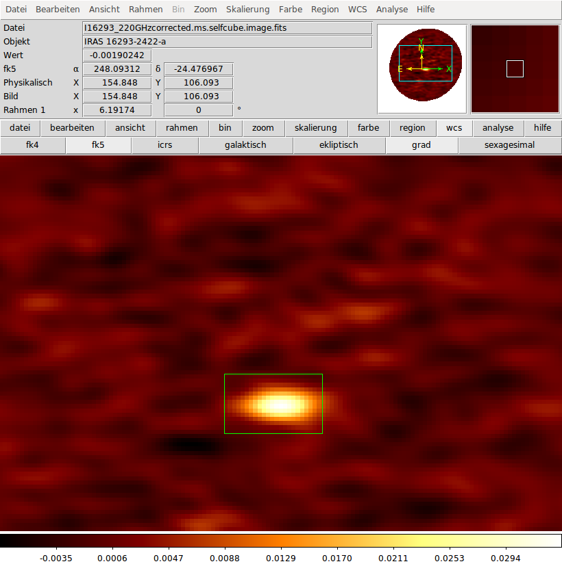
In order to fit only a part of the whole ALMA cube we need a ds9 region file which can be downloaded here. Please note, that the coordinates are given in degrees and that the shape of the region is rectangular. Additional we set the threshold parameter to 0.05, i.e. we do not fit pixels with a maximal intensity below 0.05 K.
Observational xml file
For the myXCLASSMapFit function we have to define the frequency range, (here from 220.079 to 220.313 GHz), the size of the interferometric beam FWHM (here 1.777 arcsec), the background and dust parameters. Here, we will use the following observational xml file called observation_map__Band_6.xml
    1


        IRAS16293_Band6_ReferenceImages/I16293_220GHzcorrected.ms.selfcube.image.fits


        xclassFITS


        1


            2.20079e+5
            2.20313e+5
            0.1


            True
            0.0
            0.0


            True
            1.0E+24
            0.0
            0.0


        0.0


        1.7769575715066


        True


    True
    map-molecules__Band_6__iso-ratio_file.dat
molfit and iso ratio file
Now, we have to define a molfit file describing which molecules are taken into account and how many components are used for each molecule. But how do we identify the molecules which are included in the current frequency range? First of all we have to extract one characteristic spectrum from the region which contains more or less all lines. In general it is necessary to fit different pixel spectra to create a molfit file which can be used as initial guess for all pixel of the selected region. Now we have to identify the molecules included in the selected spectrum. One possibility is to use the GetTransition function and identify the molecules which have the strongest transitions with the lowest lower energies. Another possibility is to apply the LineID function. Here, we used the GetTransition function because the frequency range is quite narrow so that the LineID function would not produce reliable results. We identify three molecules: "CH3OCHO, v=0" with two velocity components at 0.9 and 2.2 km/s, "HCOCH2OH, v=0" with one velocity component at 5.0 km/s, and "C2H5OH, v=0" with one velocity component at 0.3 km/s.
% Number of molecules 1
% schema:
%
% name of molecule   number of components
%  f:  low:     up:    s_size:   f:  low:      up:      T_rot:   f:      low:       up:        N_tot:   f:  low:    up:  V_width:   f:    low:    up:    V_off:    AFlag:
%
CH3OCHO;v=0;   2
    n  1.00  500.00   100.0000    y  3.00  1000.00   218.15093    y  1.00e+11  1.00e+19   1.38500e+14    y  0.50  10.00   1.57708    y  -50.00  50.00   0.93089    c
    n  1.00  500.00   100.0000    y  3.00  1000.00   262.05873    y  1.00e+11  1.00e+19   7.92441e+14    y  0.50  10.00   9.83775    y  -50.00  50.00   2.21164    c
HCOCH2OH;v=0;   1
    n  1.00  500.00   100.0000    y  3.00  1000.00   100.00000    y  1.00e+11  1.00e+16   3.00000e+13    y  0.50  10.00   8.00000    y  -50.00  50.00   5.00000    c
C2H5OH;v=0;   1
    n  1.00  500.00   100.0000    y  3.00  1000.00   849.40001    y  1.00e+11  1.00e+16   6.04087e+14    y  0.50   9.00   8.34149    y  -50.00  50.00   0.32545    c
The molfit file "map-molecules__Band_6__all-molecules.molfit" used for this tutorial can also be downloaded here.
In addition we take the following isotopologues and vibrational excited molecules into account "CH3O13CHO, v=0", "CH3O13CHO, v18=1", "CH3OCHO, v18=1", "C2H513CN, v=0", "C2H3CN, v11=1", "C2H3CN, v15=1", "HCOCH2OH, v12=1", "HCOCH2OH, v17=1", "HCOCH2OH, v18=1" by using the iso ratio file "map-molecules__Band_6__iso-ratio_file.dat",
% Isotopologue:                       Iso-master:              Iso-ratio:              Lower-limit:              Upper-limit:
CH3OC-13-HO;v18=1;                    CH3OCHO;v=0;                  28.00                      1.00                      1.00
CH3OCHO;v18=1;                        CH3OCHO;v=0;                   1.00                      1.00                      1.00
CH3OC-13-HO;v=0;                      CH3OCHO;v=0;                  28.00                      1.00                      1.00
C2H3CN;v11=1;                         C2H3CN;v=0;                    1.00                      1.00                      1.00
C2H3CN;v15=1;                         C2H3CN;v=0;                    1.00                      1.00                      1.00
C2H5C-13-N;v=0;                       C2H5CN;v=0;                   28.00                      1.00                      1.00
HCOCH2OH;v18=1;                       HCOCH2OH;v=0;                  1.00                      1.00                      1.00
HCOCH2OH;v17=1;                       HCOCH2OH;v=0;                  1.00                      1.00                      1.00
HCOCH2OH;v12=1;                       HCOCH2OH;v=0;                  1.00                      1.00                      1.00
which can be downloaded here. Note, we set the ratio between molecules and vibrational excited molecules to one and assume a 12C/13C ratio of 28.
algorithm xml file
In order to fit the parameters we used in the molfit and the iso ratio file we have to define the optimization algorithm(s) which is (are) used by the myXCLASSMapFit function. Here, we use the default optimization algorithm i.e. the Levenberg-Marquardt algorithm. We want to limit the max. number of iterations per pixel to 15 by setting the input parameter NumberIteration to 15, i.e. NumberIteration = 15.
Call myXCLASSMapFit function
Now everything is prepared to start the myXCLASSMapFit function. Note, we do not use a cluster file here, i.e. we use only one computer and do not use fit results from the previous row.
Within CASA
In CASA the myXCLASSMapFit function is started by
# In CASA:
MolfitsFileName = "map-molecules__Band_6__all-molecules.molfit"
experimentalData = "my_observation__map.xml"
NumberIteration = 15
regionFileName = "region_small__Band_6.reg"
UsePreviousResults = False
clusterdef = ""
JobDir = myXCLASSMapFit()
Without CASA
Use the following python script if XCLASS is used without CASA,
#!/usr/bin/python
# -*- coding: utf-8 -*-

# import sys package
import sys

# get environment variable for XCLASS root directory
XCLASSRootDir = str(os.environ.get('XCLASSRootDir', ''))
XCLASSRootDir = XCLASSRootDir.strip()
if (XCLASSRootDir != ""):
    NewModulesPaths = [XCLASSRootDir + "/build_tasks/"]
else:
    # use the following line to define XCLASS root directory manually
    NewModulesPath = "path-of-XCLASS-Interface/build_tasks/"

# extend sys.path variable
already_included_flag = False
for entries in sys.path:
    if (entries == NewModulesPath):
        already_included_flag = True
        break
    if (not already_included_flag):
        sys.path.append(NewModulesPath)

# import module task_myXCLASSMapFit
import task_myXCLASSMapFit

# define parameters for myXCLASSMapFit function

# define path and name of molfit file
MolfitsFileName = LocalPath + "map-molecules__Band_6.molfit"

# define optimization algorithm parameters
NumberIteration = 15
AlgorithmXMLFile = ""

# define path and name of obs. xml file
experimentalData = LocalPath + "observation_map__Band_6___FITS__stand-alone.xml"

# define region
regionFileName = LocalPath + "region_small__Band_6.reg"

# define telescope parameters
TelescopeSize = 1.7769575715066
Inter_Flag = True
FreqMin = 0.0
FreqMax = 0.0
RestFreq = 0.0
vLSR = 0.0

# define threshold
Threshold = 0.05

# define continuum parameters
t_back_flag = True
tBack = 0.0
tslope = 0.0
nH_flag = True
N_H = 3.E+20
beta_dust = 1.4
kappa_1300 = 0.0

# define iso ratio file parameters
iso_flag = True
IsoTableFileName = LocalPath + ""

# fit parameters param
UsePreviousResults = False
clusterdef = ""

# start myXCLASSMapFit function
JobDir = task_myXCLASSMapFit.myXCLASSMapFit(NumberIteration, AlgorithmXMLFile, MolfitsFileName, experimentalData, \
                                            regionFileName, UsePreviousResults, Threshold, FreqMin, FreqMax, \
                                            TelescopeSize, Inter_Flag, t_back_flag, tBack, tslope, nH_flag, N_H, \
                                            beta_dust, kappa_1300, iso_flag, IsoTableFileName, RestFreq, vLSR, \
                                            clusterdef)
Results
After finishing the fits of the selected pixels the myXCLASSMapFit function produces a couple of FITS images describing the optimized fit parameters for each pixel and the quality of the each pixel fit.
For "CH3OCHO, v=0" we get for the excitation temperature of the first componen
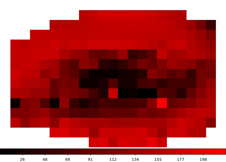
Note, the white pixels corresponds to pixels which are not fitted.
The myXCLASSMapRedoFit function can be used to improve the fit of a certain pixel.